Constrained Dynamics (IV)
This post is a direct continuation to the latest entry…
- Part III: Constrained Dynamics (III) - Force-based constraints.
…and the rest of the series:
- Part II: Constrained Dynamics (II) - Don’t use springs to model rigid constraints.
- Part I: Constrained Dynamics (I) - Unconstrained dynamics.
Let’s continue where we left off and find a more compact vector/matrix form for force-based constraints.
Generic constraints (vector form)
Everything we discussed in the previous post for the (unit circle) distance constraint can be extrapolated to generic motion, as long as we can define the trajectory as a (gradient) function \(C\) of the state of the particle:
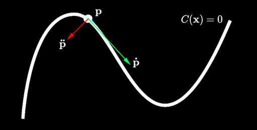
\(C\) is called position constraint and is satisfied only when \(C(\mathbf{x}=\mathbf{p})=0\).
What comes next is derived from the previous post.
In vector form:
\[\mathbf{p}=\begin{bmatrix}x\\y\end{bmatrix},\mathbf{\dot{p}}=\begin{bmatrix}\dot{x}\\\dot{y}\end{bmatrix}\]Via the chain rule the expression for the velocity constraint \(\dot{C}\) is:
\[\dot{C}=\frac{\mathrm{d}\mathbf{C}}{\mathrm{d}t}=\frac{\partial{\mathbf{C}}}{\partial{\mathbf{p}}}\frac{\mathrm{d}\mathbf{p}}{\mathrm{d}t}=\mathbf{J}\mathbf{\dot{p}}+b=0\]Where \(\mathbf{J}=\frac{\partial{\mathbf{C}}}{\partial{\mathbf{p}}}\) (called the Jacobian) is a row vector perpendicular to \(\mathbf{\dot{p}}\). The bias \(b\) is a residual term which may be used to model velocity-inducing constraints (e.g., a motor like in the animation below).
If \(\mathbf{J}\) is perpendicular to \(\mathbf{\dot{p}}\) then it is co-linear to the trajectory’s normal, which happens to be the direction of the corrective force:
\[\mathbf{F_c}=\mathbf{J}^T\lambda\]\(\lambda\) is a scalar that gives orientation/magnitude to \(\mathbf{F_c}\) known as Lagrange multiplier.
Via the chain rule again the expression for the acceleration constraint \(\ddot{C}\) is:
\[\ddot{C}=\mathbf{\dot{J}}\mathbf{\dot{p}}+\mathbf{J}\mathbf{\ddot{p}}=0\]We expect constraint forces to do no work (principle of virtual work). Since power is force times velocity:
\[P_c=\mathbf{F_c}\cdot\mathbf{\dot{p}}=\mathbf{F_c}^T\mathbf{\dot{p}}=0\implies(\lambda\mathbf{J}^T)^T\mathbf{\dot{p}}=(\mathbf{J}\mathbf{\dot{p}})\lambda=0\]Which is indeed 0 for \(\dot{C}=0,b=0\) (see above).
Plugging in Newton’s 2nd Law (\(\mathbf{F}=m\mathbf{\ddot{p}}\)):
\[\ddot{C}=\mathbf{\dot{J}}\mathbf{\dot{p}}+\mathbf{J}\frac{\mathbf{F_a}+\mathbf{F_c}}{m}=\mathbf{\dot{J}}\mathbf{\dot{p}}+\frac{\mathbf{J}\mathbf{F_a}}{m}+\frac{\mathbf{J}\mathbf{J}^T}{m}\lambda=0\]Let’s define \(w=m^{-1}\) to end up with this linear equation, where only \(\lambda\) is unknown:
\[\mathbf{J}w\mathbf{J}^T\lambda=-(\mathbf{\dot{J}}\mathbf{\dot{p}}+\mathbf{J}w\mathbf{F_a})\]We won’t simplify this beauty any further to later appreciate the parallelism with its matrix form.
Once we solve for \(\lambda\) we must apply \(\mathbf{F}=\mathbf{F_a}+\mathbf{J}^T\lambda\) to the particle to find \(\mathbf{\ddot{p}}\), then update \(\mathbf{\dot{p}}\) and \(\mathbf{p}\), and be done!
Example: Distance constraint
The recipe to find \(\mathbf{J}\) is to derive the position constraint \(C\) expressed in vector form into \(\dot{C}\), and then rearrange the resulting expression until it resembles \(\mathbf{J}\mathbf{\dot{p}}+b\).
We shall borrow the expression for \(C\) from the previous post:
\[\begin{flalign} & && C=\frac{1}{2}(\mathbf{p}\cdot\mathbf{p}-1) & \\ & && \dot{C}=\mathbf{p}\cdot\mathbf{\dot{p}}=\mathbf{J}\mathbf{\dot{p}}+0 & \\ & && \mathbf{J}=\mathbf{p}^T & \\ & && \mathbf{\dot{J}}=\mathbf{\dot{p}}^T & \end{flalign}\]Hooray! \(\lambda\) matches what we obtained back then:
\[\lambda=-\frac{m\mathbf{\dot{J}}\mathbf{\dot{p}}+\mathbf{J}\mathbf{F_a}}{\mathbf{J}\mathbf{J}^T}=-\frac{\mathbf{\dot{p}}\cdot\mathbf{F_a}+m\mathbf{\dot{p}}\cdot\mathbf{\dot{p}}}{\mathbf{p}\cdot\mathbf{p}}\]Systems of constraints (matrix form)
So far we’ve dealt with just one particle and one constraint. But what happens when there are multiple particles subjected to multiple constraints? Well… things gets a bit more involved; especially if the constraints define relationships between two or more particles at once (e.g., keep two particles a specified distance apart, etc…).
Like above, the goal is to calculate one \(\lambda_i\) for each constraint and apply the corresponding constraint forces. But intuition (correctly) says that we must solve for all the \(\lambda_i\) simultaneously and not one by one. This makes sense, because otherwise satisfying one constraint at a time, isolated from the rest, would potentially violate all the others, and so on.
This looks like a job for a (large) system of linear equations solver!
Please bear with me in the derivation:
- Concat all the \((x,y)\) particle positions in a long column \(\mathbf{q}\) called state vector.
- Define a diagonal matrix \(\mathbf{M}\) with all the particle masses. Define \(\mathbf{W}=\mathbf{M}^{-1}\).
- Define two long column vectors \(\mathbf{Q_a}\) and \(\mathbf{Q_c}\) where all the force components (\(\mathbf{F_a}\) and \(\mathbf{F_c}\) respectively) are concatenated.
- Define the super-constraint \(\mathbf{C}(\mathbf{q})\) as a function of the (concatenated) particle states.
- By the chain rule:
- By the chain rule again:
- By Newton’s 2nd Law:
- By substitution:
- By the principle of virtual work (perpendicular/co-linear like above):
- By substitution:
This last expression is a (potentially large) system of linear equations where the vector \(\mathbf{\lambda}\) is the only unknown.
Once we solve for \(\mathbf{\lambda}\) we must apply \(\mathbf{Q}=\mathbf{Q_a}+\mathbf{J}^T\mathbf{\lambda}\) to find \(\mathbf{\ddot{q}}\), then update \(\mathbf{\dot{q}}\) and \(\mathbf{q}\), and be done!
Wonderful. Isn’t it?
Summary (particles)
For \(n\) particles and \(m\) constraints:
\[\mathbf{q}=\begin{bmatrix}{p_1}_x\\{p_1}_y\\{p_2}_x\\{p_2}_y\\ \vdots\\{p_n}_x\\{p_n}_y\end{bmatrix},\mathbf{\dot{q}}=\begin{bmatrix}\dot{p_1}_x\\ \dot{p_1}_y\\ \dot{p_2}_x\\ \dot{p_2}_y\\ \vdots\\ \dot{p_n}_x\\ \dot{p_n}_y\end{bmatrix},\mathbf{Q_a}=\begin{bmatrix}{\mathbf{Q_a}_1}_x\\{\mathbf{Q_a}_1}_y\\{\mathbf{Q_a}_2}_x\\{\mathbf{Q_a}_2}_y\\ \vdots\\{\mathbf{Q_a}_n}_x\\{\mathbf{Q_a}_n}_y\end{bmatrix},\mathbf{W}=\begin{bmatrix}m_1& & & & & &\\&m_1& & & & &\\& &m_2& & & &\\& & &m_2& & &\\& & & &\ddots& &\\& & & & &m_n&\\& & & & & &m_n\end{bmatrix}\] \[\mathbf{J}=\begin{bmatrix} \frac{\partial{\mathbf{C_1}_x}}{\partial{\mathbf{q_1}_x}}& \frac{\partial{\mathbf{C_1}_x}}{\partial{\mathbf{q_1}_y}}& \frac{\partial{\mathbf{C_1}_x}}{\partial{\mathbf{q_2}_x}}& \frac{\partial{\mathbf{C_1}_x}}{\partial{\mathbf{q_2}_y}}&\dots& \frac{\partial{\mathbf{C_1}_x}}{\partial{\mathbf{q_n}_x}}& \frac{\partial{\mathbf{C_1}_x}}{\partial{\mathbf{q_n}_y}}\\ \frac{\partial{\mathbf{C_1}_y}}{\partial{\mathbf{q_1}_x}}& \frac{\partial{\mathbf{C_1}_y}}{\partial{\mathbf{q_1}_y}}& \frac{\partial{\mathbf{C_1}_y}}{\partial{\mathbf{q_2}_x}}& \frac{\partial{\mathbf{C_1}_y}}{\partial{\mathbf{q_2}_y}}&\dots& \frac{\partial{\mathbf{C_1}_y}}{\partial{\mathbf{q_n}_x}}& \frac{\partial{\mathbf{C_1}_y}}{\partial{\mathbf{q_n}_y}}\\ \frac{\partial{\mathbf{C_2}_x}}{\partial{\mathbf{q_1}_x}}& \frac{\partial{\mathbf{C_2}_x}}{\partial{\mathbf{q_1}_y}}& \frac{\partial{\mathbf{C_2}_x}}{\partial{\mathbf{q_2}_x}}& \frac{\partial{\mathbf{C_2}_x}}{\partial{\mathbf{q_2}_y}}&\dots& \frac{\partial{\mathbf{C_2}_x}}{\partial{\mathbf{q_n}_x}}& \frac{\partial{\mathbf{C_2}_x}}{\partial{\mathbf{q_n}_y}}\\ \frac{\partial{\mathbf{C_2}_y}}{\partial{\mathbf{q_1}_x}}& \frac{\partial{\mathbf{C_2}_y}}{\partial{\mathbf{q_1}_y}}& \frac{\partial{\mathbf{C_2}_y}}{\partial{\mathbf{q_2}_x}}& \frac{\partial{\mathbf{C_2}_y}}{\partial{\mathbf{q_2}_y}}&\dots& \frac{\partial{\mathbf{C_2}_y}}{\partial{\mathbf{q_n}_x}}& \frac{\partial{\mathbf{C_2}_y}}{\partial{\mathbf{q_n}_y}}\\ \vdots& \vdots& \vdots& \vdots&\ddots& \vdots& \vdots\\ \frac{\partial{\mathbf{C_m}_x}}{\partial{\mathbf{q_1}_x}}& \frac{\partial{\mathbf{C_m}_x}}{\partial{\mathbf{q_1}_y}}& \frac{\partial{\mathbf{C_m}_x}}{\partial{\mathbf{q_2}_x}}& \frac{\partial{\mathbf{C_m}_x}}{\partial{\mathbf{q_2}_y}}&\dots& \frac{\partial{\mathbf{C_m}_x}}{\partial{\mathbf{q_n}_x}}& \frac{\partial{\mathbf{C_m}_x}}{\partial{\mathbf{q_n}_y}}\\ \frac{\partial{\mathbf{C_m}_y}}{\partial{\mathbf{q_1}_x}}& \frac{\partial{\mathbf{C_m}_y}}{\partial{\mathbf{q_1}_y}}& \frac{\partial{\mathbf{C_m}_y}}{\partial{\mathbf{q_2}_x}}& \frac{\partial{\mathbf{C_m}_y}}{\partial{\mathbf{q_2}_y}}&\dots& \frac{\partial{\mathbf{C_m}_y}}{\partial{\mathbf{q_n}_x}}& \frac{\partial{\mathbf{C_m}_y}}{\partial{\mathbf{q_n}_y}}\\ \end{bmatrix},\mathbf{\dot{J}}=\frac{\mathrm{d}\mathbf{J}}{\mathrm{d}t}\]The state and force vectors are \(2n\) elements tall. The Jacobian matrices are \(2m\) elements tall and \(2n\) elements wide.
In this summary I am assuming that each constraint yields one (and only one) corrective force, with two \((x,y)\) components as is the case in the constraints discussed so far. More complicated contraints may contribute more than two components, making \(\mathbf{J}\) be taller.
Countering drift
We may inject a spring-y term in \(\mathbf{\ddot{C}}=0\) resulting in this monstrosity:
\[\mathbf{J}\mathbf{W}\mathbf{J}^T\mathbf{\lambda}=-(\mathbf{\dot{J}}\mathbf{\dot{q}}+\mathbf{J}\mathbf{W}\mathbf{Q_a}+k_s\mathbf{C}+k_d\mathbf{\dot{C}})\]As explained in the previous post, these extra terms will make sure that particles “spring back” to legal positions as soon as they attempt to drift away.
Extension to rigid bodies
So far we’ve used point-mass particles. But the extension to 2D rigid bodies is fairly easy:
- Rotation aside, a rigid body behaves exactly as a point-mass positioned at its center-of-mass.
- Position \(\mathbf{p}\) vs. angle \(\theta\), linear \(\mathbf{\dot{p}}\) vs. angular \(\dot{\theta}\) velocity, linear \(\mathbf{\ddot{p}}\) vs. angular \(\ddot{\theta}\) acceleration, and mass \(m\) vs. moment-of-inertia \(I\) all exhibit analogous behavior. In particular, Newton’s 2nd Law applied to angular motion states that:
A body’s moment of inertia \(I\) defines how hard it is for a rotational force \(\tau\) (called torque) to induce a change in its angular acceleration \(\ddot{\theta}\). Just like mass \(m\) defines how hard it is for a linear force \(\mathbf{F}\) to induce a change in the body’s linear acceleration:
\[\mathbf{F}=m\mathbf{\ddot{p}}\]In our code we must extend the particle state struct \([\mathbf{p}, \mathbf{\dot{p}}]\) to the body state struct \([\mathbf{p}, \theta, \mathbf{\dot{p}}, \dot{\theta}]\).
The \(I\) of a rigid body is a characteristic of its shape and mass distribution. Simple shapes such as disks and rectangles have well-known expressions as long as their density is homogeneous.
Summary (rigid bodies)
This parallelism between angular/linear makes it easy to extend our matrix form to support torque/rotation alongside linear force/position.
\[\mathbf{q}=\begin{bmatrix}{p_1}_x\\{p_1}_y\\ \theta_1\\{p_2}_x\\{p_2}_y\\ \theta_2\\ \vdots\\{p_n}_x\\{p_n}_y\\ \theta_n\end{bmatrix},\mathbf{\dot{q}}=\begin{bmatrix}\dot{p_1}_x\\ \dot{p_1}_y\\ \dot{\theta_1}\\ \dot{p_2}_x\\ \dot{p_2}_y\\ \dot{\theta_2}\\ \vdots\\ \dot{p_n}_x\\ \dot{p_n}_y\\ \dot{\theta_n}\end{bmatrix},\mathbf{Q_a}=\begin{bmatrix}{\mathbf{Q_a}_1}_x\\{\mathbf{Q_a}_1}_y\\ \tau_1\\{\mathbf{Q_a}_2}_x\\{\mathbf{Q_a}_2}_y\\ \tau_2\\ \vdots\\{\mathbf{Q_a}_n}_x\\{\mathbf{Q_a}_n}_y\\ \tau_n\end{bmatrix},\mathbf{W}=\begin{bmatrix}m_1& & & & & & & & &\\&m_1& & & & & & & &\\& &I_1& & & & & & &\\& & &m_2& & & & & &\\& & & &m_2& & & & &\\& & & & &I_2& & & &\\& & & & & &\ddots& & &\\& & & & & & &m_n& &\\& & & & & & & &m_n&\\& & & & & & & & &I_n\end{bmatrix}^{-1}\]And likewise for \(\mathbf{J}\) and \(\mathbf{\dot{J}}\), which also must involve \(\theta_i\) and \(\tau_i\).
The state and force vectors are now \(3n\) elements tall. The Jacobian matrices are now \(2m\) elements tall and \(3n\) elements wide.
My implementation
I have recently implemented all this into my beloved Topotoy engine.
This contraption below is a force-based rigid-body simulation where there is a motorized constraint, and then a bunch of different constraints I support: spring, distance, and rack-and-pinion. Everything is coded exactly as described in this post.
As one might expect, accurate-and-efficient implementation of this all brings its own universe of challenges and opportunities for exploration. So… down the rabbit-hole I went.
Each of these subjects below is worth their own blog post, but for the sake of brevity I will not get into that much detail here.
Large SLE solvers
The size of all the vectors and matrices involved grows \(O(n)\) and \(O(n^2)\) respectively with the number of bodies/constraints in the system. This very quickly poses a problem both in storage space and more so in efficiency.
I’ve tried Gauss-Seidel, Gaussian Elimination, and the Conjugate Gradient method. The CG method in particular benefits from the fact that \(\mathbf{J}\) is very sparse (read below).
Efficient and numerically-robust implementation of these methods is definitely a meaty subject itself.
Sparse matrices
The matrix \(\mathbf{W}\) is all zeros except for the diagonal, so it can be stored as a vector. Multiplying by \(\mathbf{W}\) can be coded as a simple per-row scalar multiplication instead of a full-fledged \(O(n^4)\) matrix product.
But the most relevant observation here is that \(\mathbf{J}\) is a sparse matrix.
Constraints usually define a relationship between 2 bodies. This makes rows \(2i,2i+1\) for constraint \(\mathbf{C_i}\) contain only \(6=2\times\{m,m,I\}\) non-zero coefficients each because the coefficients corresponding to bodies not affected by \(\mathbf{C_i}\) are constant (0 derivative) with respect to the state of those bodies.
In our particular case, matrix sparsity is aligned in blocks of 3 coefficients because of the \(\{m,m,I\}\) arrangement. The implementation can exploit this knowledge to give proper column block granularity.
Actually, the way in which each constraint contributes its own coefficients to the large matrices \(\mathbf{J},\mathbf{\dot{J}}\) goes like this:
- Start with a blank sparse matrix.
- For each constraint \(\mathbf{C_i}\):
- Compute the constraint’s own \(\mathbf{J}\) 6 (3 coeffs x 2 bodies) coefficients.
- Allocate two 3x1 blocks per row in the large \(\mathbf{J}\) at the right locations.
- Fill those in with a copy of the constraint’s coefficients.
- Do the same for \(\mathbf{\dot{J}}\).
Sparse matrices bring some big opportunities for optimization. For example, the product of 2 sparse matrices can skip the zero’d blocks and approach \(O(n^2)\) complexity instead of \(O(n^4)\) the higher the proportion of zero vs. non-zero elements becomes.
Remarkably, \(\mathbf{J}\mathbf{W}\mathbf{J}^T\) happens to be sparse as well (and also symmetric). This encourages the use of the Conjugate Gradient method for the SLE solver. This algorithm solves \(\mathbf{L}\mathbf{\lambda}=\mathbf{R}\) iteratively in way that preserves sparsity of the operands involved all the way through. This is unlike general methods such as GS or GE where sparsity is not exploited and the large size of the matrices involved becomes a serious drag performance-wise.
ODE solvers
I’ve tried semi-implicit Euler and Runge-Kutta 4 so far. Simulations withstand more stress with RK4, clearly.
Coming soon…
The next and last chapter in this series will be about the impulse-based approach, which is the method used by (among others) the widely-popular box2d library.
I am currently in the process of supporting impulse-based dynamics (alongside force-based) in my engine myself. So I intend to document the process a little bit very soon.
Stay tuned!
P.S.: Apologies for any typos, imprecisions or mistakes there may be in this series. >.<