Constrained Dynamics (III)
This post is a continuation to the first two entries in this series:
- Part II: Constrained Dynamics (II) - Don’t use springs to model rigid constraints.
- Part I: Constrained Dynamics (I) - Unconstrained dynamics.
Constrained dynamics (recap)
In a system where masses (particles) are ruled by newtonian dynamics (forces/accelerations), “constrained dynamics” is the ability to enforce custom restrictions on the way the particles are permitted to move.
For example, we might constrain a particle to follow a given path, or keep a certain distance from a fixed point in space, or make two particles stay a specified distance apart. In other words: remove degrees of freedom of movement.
The goal is to enforce these constraints strictly within the framework of newtonian dynamics, where forces are the only agent that induces a change of state (via acceleration). So our job here is to directly calculate the corrective forces required to satisfy the constraints at all times.
There are different ways to achieve this, but in this mini-series we will focus on these two:
- Force-based constraints: Which works in the acceleration realm (2nd derivative).
- Impulse-based constraints: Which works in the velocity realm (1st derivative).
Actually, this post describes the force-based dynamics approach.
Nomenclature
We will distinguish between:
- \(\mathbf{F_a}\) - Applied forces. Such as gravity, wind, or other user-interaction forces.
- \(\mathbf{F_c}\) - Constraint forces. Forces we will calculate ourselves in order to satisfy the constraints.
Particles are affected by the sum of both.
The job of the constraint forces is to cancel out those components of the applied forces that act against the constraints. This in turn makes sure that the resulting particle accelerations are consistent with the constraints.
Example: Distance constraint
We will use again a distance constraint as an example, where we have one particle under the effect of gravity, which motion is restricted to the unit circle. You can picture this as an ideal pendulum where the particle hangs by a unit-length mass-less thread pinned to the origin.
In its simplest form, a constraint is any function \(C\) of the state \(\mathbf{x}\) of the particle.
An equality constraint is said to be satisfied only when \(C(\mathbf{x})=0\).
The expression of the unit circle distance constraint can be written as:
\[C(\mathbf{x})=\sqrt{\mathbf{p}\cdot\mathbf{p}}-1=0\]Which is derived from the implicit equation of the circle (\(r=1\)):
\[\mathbf{p}\cdot\mathbf{p}=x^2+y^2=r^2=1^2\]Geometric intuition
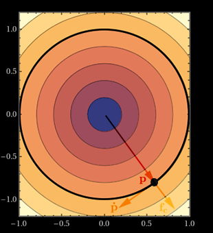
Our \(C(\mathbf{x})\) happens to be a Signed Distance Function which radiates away from the origin, perpendicular to the unit circle (in black):
If we plot \(z=C(x,y)=\sqrt{x^2+y^2}-1\) in Wolfram Alpha we get this surface:
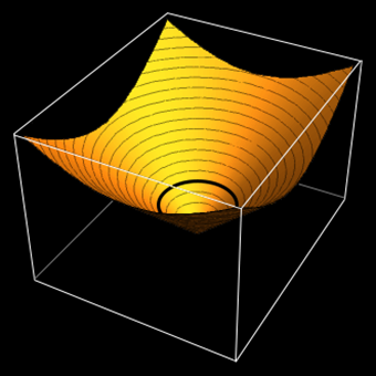
This is called the constraint hypersurface, and can be understood as a gradient field. Any constraint you may specify has its own characteristic hypersurface.
In our case, the hypersurface is a cone and the subset of legal positions for the particle (\(C=0\)) is highlighted as a black ring.
We would expect that if \(\mathbf{p}\) is on the black ring, then the only legal velocities \(\mathbf{\dot{p}}\) would be tangential, causing no increase/decrease along the gradient \(C\) whatsoever.
Likewise, whenever the particle attempts to abandon the black ring, the corrective constraint force \(\mathbf{F_c}\) would act on the particle in a direction perpendicular to the ring, causing maximum corrective increase/decrease along the gradient \(C\).
Trick: We can find an equivalent expression for \(C\) by using squared distances, or multiplying by a constant. Why do this? Well, we may want to get rid of the square root so the derivatives we will be calculating next will be greatly simplified:
\[C(\mathbf{x})=\frac{1}{2}(\mathbf{p}\cdot\mathbf{p}-1)=0\]In doing so the constraint hypersurface becomes a paraboloid instead of a cone. But everything discussed so far remains the same.
Deriving \(C\) w.r.t. time
If the position constraint \(C\) is 0 then the particle is on the unit circle, at a legal position. Over time, the only permitted walk through the constraint hypersurface is such that \(C = 0\) is never violated:
\[\begin{flalign} C = 0 \\ \dot{C} = 0 \\ \ddot{C} = 0 \end{flalign}\]Reminder: The derivative of the dot product of two vectors is given by:
\[\frac{\mathrm{d}(\mathbf{u}(t)\cdot\mathbf{v}(t))}{\mathrm{d}t}=\mathbf{u}(t)\cdot\frac{\mathrm{d}\mathbf{v}(t)}{\mathrm{d}t}+\frac{\mathrm{d}\mathbf{u}(t)}{\mathrm{d}t}\cdot\mathbf{v}(t)\]So the velocity constraint is:
\[\dot{C}=\frac{\mathrm{d}{\frac{1}{2}(\mathbf{p}\cdot\mathbf{p}-1)}}{\mathrm{d}t}=\frac{1}{2}(\mathbf{p}\cdot\mathbf{\dot{p}}+\mathbf{\dot{p}}\cdot\mathbf{p})=\mathbf{p}\cdot\mathbf{\dot{p}}=0\]This coincides with the above geometrical intuition: legal velocities must be perpendicular to legal position vectors. i.e., tangential to the unit circle.
The acceleration constraint is:
\[\ddot{C}=\frac{\mathrm{d}{(\mathbf{p}\cdot\mathbf{\dot{p}})}}{\mathrm{d}t}=\mathbf{p}\cdot\mathbf{\ddot{p}}+\mathbf{\dot{p}}\cdot\mathbf{\dot{p}}=0\]Solving for \(\mathbf{F_c}\)
By Newton’s 2nd Law:
\[\mathbf{F}=\mathbf{F_a}+\mathbf{F_c}=m\ddot{\mathbf{p}}\]Which we can combine with \(\ddot{C}\):
\[\ddot{C}=\mathbf{p}\cdot\frac{\mathbf{F_a}+\mathbf{F_c}}{m}+\mathbf{\dot{p}}\cdot\mathbf{\dot{p}}=0\]Only the constraint force is unknown, so let’s try and isolate \(\mathbf{F_c}\):
\[\mathbf{p}\cdot\mathbf{F_c}=-(\mathbf{p}\cdot\mathbf{F_a}+m\mathbf{\dot{p}}\cdot\mathbf{\dot{p}})\]Note that because \(\mathbf{F_c}\) is a 2D vector, this is really one equation with two unknowns: \(\mathbf{F_c}=(\mathbf{F_c}_x,\mathbf{F_c}_y)\).
Principle of virtual work
We expect constraint forces to never add or remove energy from the system.
constraint forces do no work.
Let’s take the (kinetic) energy of the particle:
\[E_k=\frac{m}{2}\mathbf{\dot{p}}\cdot\mathbf{\dot{p}}\]And its derivative w.r.t. time:
\[\dot{E_k}=\frac{m}{2}(\mathbf{\dot{p}}\cdot\mathbf{\ddot{p}}+\mathbf{\ddot{p}}\cdot\mathbf{\dot{p}})=m\mathbf{\dot{p}}\cdot\mathbf{\ddot{p}}=\mathbf{F_a}\cdot\mathbf{\dot{p}}+\mathbf{F_c}\cdot\mathbf{\dot{p}}\]We end up with the work done by \(\mathbf{F_a}\) and \(\mathbf{F_c}\), and we expect the \(\mathbf{F_c}\) part to be 0:
\[\mathbf{F_c}\cdot\mathbf{\dot{p}}=0\]Which geometrically means that legal constraint forces must be perpendicular to legal velocities, which are tangential. Which in turn means that \(\mathbf{F_c}\) must be aligned with the position vector \(\mathbf{p}\) as illustrated above.
This alignment can be expressed as \(\mathbf{F_c}=\lambda\mathbf{p}\). So now instead of two unknowns we have just one: \(\lambda\).
Solving for \(\lambda\)
Plugging back into \(\ddot{C}\) we obtain this expression where every value to the right is known:
\[\lambda=-\frac{\mathbf{p}\cdot\mathbf{F_a}+m\mathbf{\dot{p}}\cdot\mathbf{\dot{p}}}{\mathbf{p}\cdot\mathbf{p}}\]Finally (!) the total acceleration experienced by the particle is:
\[\mathbf{\ddot{p}}=\frac{\mathbf{F_a}+\lambda\mathbf{p}}{m}\]Source code
Whoa! That was an awful lot of mathematical blah-blah…
The source code implementation is a bit less intimidating, though:
struct particle_t
{
  explicit particle_t() : m( 1 ), p( 1, 0 ), v( 0 ) {}

  void step( const f64_t dt, const vec2d_c& Fa )
  {
    const   f64_t pp =  ( p * p );
    const   f64_t vv =  ( v * v );

    const   f64_t lambda = -( ( ( p * Fa ) + ( m * vv ) ) / pp );

    const vec2d_c Fc = ( p * lambda );

    const vec2d_c a  = ( ( Fa + Fc ) / m );

    v += ( a * dt );
    p += ( v * dt );
  }

    f64_t m;  // Mass.
  vec2d_c p;  // Position.
  vec2d_c v;  // Velocity.
};
This is the code in action, assuming that the particle starts at rest at a legal position in the circle.
Ouch! The distance sadly stretches away… :( What we’re witnessing here is numerical drift when iteratively solving the position ODE with the Semi-implicit Euler method. The simulation is using dt=1/60. Time resolution greatly affects the quality of the numerical solution. So let’s try with dt=1/1500 which is 25 times smaller:
The drift is certainly reduced, but not quite gone.
Using tiny dt values is terrible for performance, because then each visual frame has the burden to run many simulation steps instead of just one or only a few. And simulation steps in non-trivial setups get very performance-heavy very quickly.
Using a numerical solver that is less prone to drift may certainly help. But won’t provide a definitive answer to this problem anyway.
So let’s resort to our old friends: springs.
Countering drift
The problem with the simulations above is not just drift per se. But the fact that nothing is bringing the particle back to a legal position once it drifts away to a non-legal position. So as numerical errors make the corrective forces insufficient, the situation is never rectified.
A robust solution to drift is to patch up the formulation above so instead of solving for \(\ddot{C}=0\) we solve for \(\ddot{C}=-(k_s{C}+k_d\dot{C})\).
This expression looks familiar since \(k_s\) and \(k_d\) are damped spring (stiffness and damping) constants.
The intention here is to bring drift (\(C\neq{0}\)) back to \(C=0\) in a spring-y fashion. Choosing \(k_s\) and \(k_d\) may require some trial-and-error, but good values are not hard to find because drift is easily absorbed:
\[\lambda=-\frac{\mathbf{p}\cdot\mathbf{F_a}+m\mathbf{\dot{p}}\cdot\mathbf{\dot{p}}+k_s{C}+k_d\dot{C}}{\mathbf{p}\cdot\mathbf{p}}\]Here’s the new simulation with dt=1/600. Now the distance fluctuates but stays in the viccinity of 1:
And here’s the new simulation code:
struct particle_t
{
  explicit particle_t() : m( 1 ), p( 1, 0 ), v( 0 ) {}

  void step( const f64_t dt, const vec2d_c& Fa )
  {
    const   f64_t ks     = 1e+2;
    const   f64_t kd     = 1e-2;

    const   f64_t pp     =  ( p * p );
    const   f64_t vv     =  ( v * v );
    const   f64_t C_dot  =  ( p * v );

    const   f64_t C      =  ( ( pp - 1 ) / 2 );

    const   f64_t k      =  ( ( ks * C ) + ( kd * C_dot ) );

    const   f64_t lambda = -( ( ( p * Fa ) + ( m * vv ) + k ) ) / pp );

    const vec2d_c Fc     =  ( p * lambda );

    const vec2d_c a      =  ( ( Fa + Fc ) / m );

    v += ( a * dt );
    p += ( v * dt );
  }

    f64_t m;
  vec2d_c p;  // Position.
  vec2d_c v;  // Velocity.
};
Generalization
In the next chapter we will discuss:
- A general formulation in vector/matrix form.
- How to handle systems with multiple particles/constraints.
Stay tuned!