Constrained Dynamics (I)
I am starting a mini-series of posts that go through the mathematical derivation necessary to build a minimal physics engine with support for constrained dynamics.
This first post is about unconstrained dynamics, using a free-falling particle as an example.
Upcoming posts will describe constrained dynamics, then build a (single-constraint) pendulum, and finally a (multi-constraint) double-pendulum.
We will restrict ourselves to:
- 2D.
- Only one particle mass.
- Only one external force (gravity).
- Only one type of constraint (distance).
Rigid bodies with a surface area, collisions, contacts, frictions, etc… will be left out of the picture.
Incredibly useful links
This mini-series is nothing but a digest of knowledge that can be found in great detail here:
- Erin Catto’s Box2D publications area.
- Physically Based Modeling: Principles and Practice by Andrew Witkin and David Baraff.
In particular:
- This presentation by Erin Catto.
- These lecture notes by Andrew Witkin.
Unconstrained dynamics
By way of newtonian mechanics:
- 1st Law: The velocity (or lack thereof) of a particle remains unchanged until a force is applied to it.
- 2nd Law: When a force is applied to a particle, it experiments an acceleration of magnitude \(\frac{\|\mathbf{F}\|}{m}\) in the direction of \(\mathbf{F}\).
As a consequence of the 1st Law, we can describe the state \(\mathbf{x}\) of a particle of mass \(m\) by its position and its velocity.
As a consequence of the 2nd Law, we can’t consider acceleration to be part of the state as it only spawns for as long as an external force is applied to the particle. Force (acceleration) is actually the only agent that causes changes of state.
These three magnitudes are 2D vectors. We will use the following notation:
\[\begin{flalign} & && \mathbf{p}=position & \\ & && \dot{\mathbf{p}}=\frac{\mathrm{d}\mathbf{p}}{\mathrm{d}t}=velocity & \\ & && \ddot{\mathbf{p}}=\frac{\mathrm{d}\dot{\mathbf{p}}}{\mathrm{d}t}=\frac{\mathrm{d}^2\mathbf{p}}{\mathrm{d}t^2}=acceleration & \end{flalign}\]Momentum
Mass and velocity together lead to the definition of linear momentum:
\[\mathbf{\rho}=m\mathbf{\dot{p}}\]Another way to read the 2nd Law is that a force acting on a particle induces a change on its momentum.
\[\mathbf{F}=\frac{\mathrm{d}\mathbf{\rho}}{\mathrm{d}t}=\frac{\mathrm{d}(m\mathbf{\dot{p}})}{\mathrm{d}t}=m\mathbf{\ddot{p}}\]We can reason that momentum is a measure of the impulse (force over time) that one must exert in order to stop the particle (i.e., cancel out its current velocity).
For a steady force, this is:
\[\begin{flalign} & && \mathbf{Imp} = \int_{t_0}^{t_1}{\mathbf{F}}\mathrm{d}{t} = \mathbf{F} \Delta{t} & \\ & && \mathbf{Imp} = \int_{t_0}^{t_1}{\frac{\mathrm{d}\mathbf{\rho}}{\mathrm{d}t}}\mathrm{d}{t} = \Delta{\mathbf{\rho}} & \end{flalign}\]State over time
The evolution of the particle’s position is so ruled by the differential equation:
\[\mathbf{p}=\mathbf{p}_0+\int_{t_0}^{t_1}{(\dot{\mathbf{p}}_0+\int_{t_0}^{t_1}{\frac{\mathbf{F}}{m}}\mathrm{d}{t})}\mathrm{d}{t}\]Which can be read as: the particle position is a function of the initial state \(\mathbf{x}_0\) (at \(t=t_0\)) and the forces applied to the particle, which cause acceleration, which modifies the velocity, which modifies the position.
The classic and most intuitive way to iteratively solve the above diffential equation is the Semi-Implicit Euler method:
\[\begin{flalign} & && \ddot{\mathbf{p}}_t=\frac{\mathbf{F}}{m} & \\ & && \dot{\mathbf{p}}_{t+\Delta{t}}=\dot{\mathbf{p}}_t+\ddot{\mathbf{p}}_t\Delta{t} & \\ & && \mathbf{p}_{t+\Delta{t}}=\mathbf{p}_t+\dot{\mathbf{p}}_t\Delta{t} & \end{flalign}\]Where each iteration is meant to encompass a discrete time slice of duration \(\Delta{t}\).
These expressions can be read as:
- Calc the acceleration caused by the total sum of applied forces at time \(t\).
- Update the particle’s velocity with said acceleration (times \(\Delta{t}\)).
- Update the particle’s position with the updated velocity (times \(\Delta{t}\)).
The intricacies of numerical solvers for differential equations are outside the scope of this post. But the above method does a fine job at producing a discrete approximation to the true state over time. At least, as long as \(\Delta{t}\) is small enough. For starters \(\Delta{t}=1/60\) (60 steps per second) is a sensible choice.
Note that the smaller the \(\Delta{t}\), the more closely that we will be approximating the exact analytic solution. More accuracy sounds ideal, but the smaller the delta, the more the steps necessary to integrate over the same total time. Also, tiny deltas may drown in the muddy waters of insufficient floating-point precision. So a value that is small, but not too small, is the right choice.
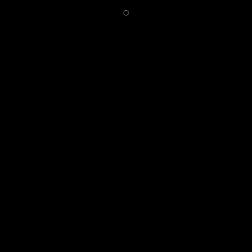
Free-fall (iterative)
We’re only considering gravity in this post (\(\mathbf{F}=\mathbf{g}\)). So the only acceleration is downwards and always steady: \(\ddot{\mathbf{p}}=\frac{\mathbf{g}}{m}\). The simulation steps become:
\[\begin{flalign} & && \dot{\mathbf{p}}_{t+\Delta{t}} = \dot{\mathbf{p}}_t + \frac{\mathbf{g}}{m} \Delta{t} & \\ & && \mathbf{p}_{t+\Delta{t}} = \dot{\mathbf{p}}_t \Delta{t} & \end{flalign}\]Here’s a simple implementation for the particle state and the simulation step:
struct particle_t
{
  explicit particle_t() : m( 1 ), p( 0 ), v( 0 ) {}

  void step( const f64_t dt, const vec2d_c& F )
  {
    const vec2d_c a = ( F / m );

    v += ( a * dt );
    p += ( v * dt );
  }

    f64_t m;  // Mass.
  vec2d_c p;  // Position.
  vec2d_c v;  // Velocity.
};
Here’s a humble animation of the particle in free-fall:
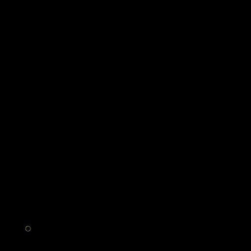
If we give an initial velocity to the particle (\(t=0\)), we end up with projectile motion:
Free-fall (analytic)
Differential equations are outside the scope of this post. But let’s say at least that an analytic solution to this example, where there’s only one steady external force, is possible and easy.
The analytic solution gives us a function that explicitly describes the position of the particle at any given time. This sounds better than an iterative simulation, although analytic solutions are untractable in non-trivial systems.
The vertical force that gravity exerts on a particle is proportional to its mass, which in turn makes gravity accelerate any particle the same regardless of its mass:
\[\mathbf{g}=\begin{bmatrix}0\\ {m}g_y\end{bmatrix}\]Plugging \(\mathbf{g}\) into the differential equation above:
\[\begin{flalign} & && x=x_0+\int_{t_0}^{t_1}{(\dot{x}_0+\int_{t_0}^{t_1}{\frac{0 }{m}}\mathrm{d}{t})}\mathrm{d}{t} & \\ & && y=y_0+\int_{t_0}^{t_1}{(\dot{y}_0+\int_{t_0}^{t_1}{\frac{m g_y}{m}}\mathrm{d}{t})}\mathrm{d}{t} & \end{flalign}\]Which analytic solution is the very familiar projectile motion formula:
\[\begin{flalign} & && x=x_0+\dot{x}_0t & \\ & && y=y_0+\dot{y}_0t+g_y{t^2} & \end{flalign}\]This type of motion is also called parabolic throw. As can be seen both in the above animation and by looking at the formula, the ballistic trajectory w.r.t. time is horizontally linear, and vertically parabolic.
Things are about to get exciting. I promise!