Fourier Transform of a unit pulse
One might need (as is the case for me now) to compute a FT without actually computing the FT. i.e., to find the explicit formulation for the resulting FT of a certain 2D signal.
In particular, as part of some optimizations in Maverick Render I wish to create a map that looks like the diffraction pattern of a polygonal aperture shape, but without computing the FT of said aperture.
From a previous post
Looking at this video from my previous post, intuition says that each of the streaks of a diffraction pattern is “kind of independent from” or “overlaps onto” the rest and could be modeled on its own from a 1D FT. This intuition is incorrect in the general case. But let’s focus on the one case where this reasoning is correct: the diffraction pattern of a square shape.
Separability of the FT
The Fourier Transform is separable in both directions:
- The 2D analysis formula can be written as a 1D analysis in the
xdirection followed by a 1D analysis in the ` y` direction. - The 2D synthesis formula can be written as a 1D analysis in the
udirection followed by a 1D analysis in the ` v` direction.
So it seems natural to focus on the 1D case first and then combine 2x 1D transforms for the square. The cross section of a square is (one cycle of) a 1D rectangular pulse.
Fourier Transform of a 1D unit pulse
From Wikipedia
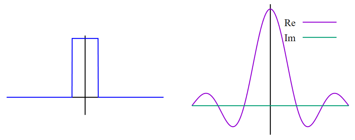
A unit pulse of amplitude A and width T is a function g(t) that yields A for t IN [-T/2..+T/2] and 0 everywhere else. Plugging this g(t) in the definition of the Fourier Transform, we obtain this:
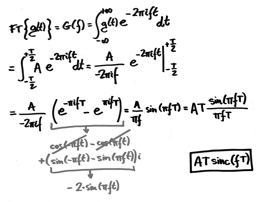
So the FT of a unit pulse is the real-valued function A*T*sinc(f*T). The imaginary component in this case cancels out.
The sinc function
The sin(pi*f*T)/(pi*f*T) part of the solution is such a fundamental building block in the field of signal processing that it got a name of its own: The venerable sinc function, or alternatively the sampling function.
From Wikipedia: The normalized sinc function is the Fourier Transform of the rectangular function with no scaling. It is used in the concept of reconstructing a continuous bandlimited signal from uniformly spaced samples of that signal.
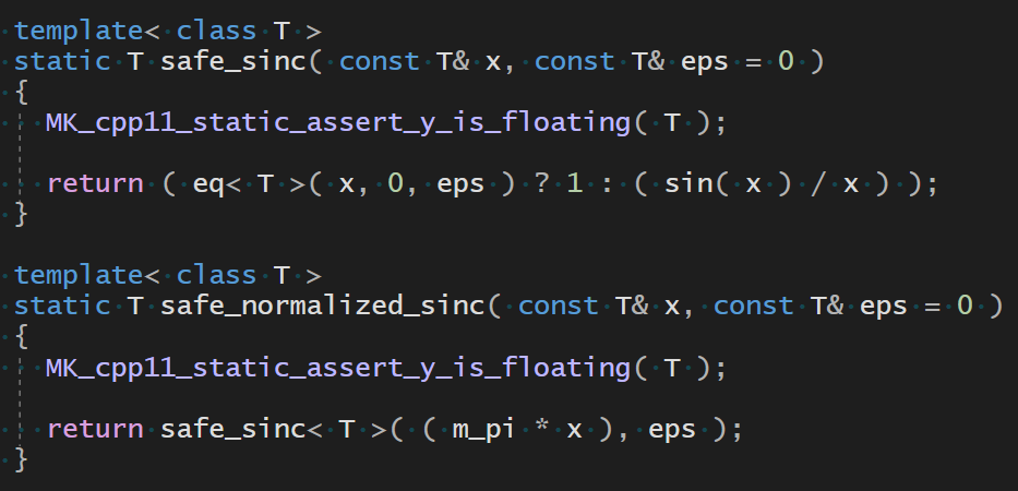
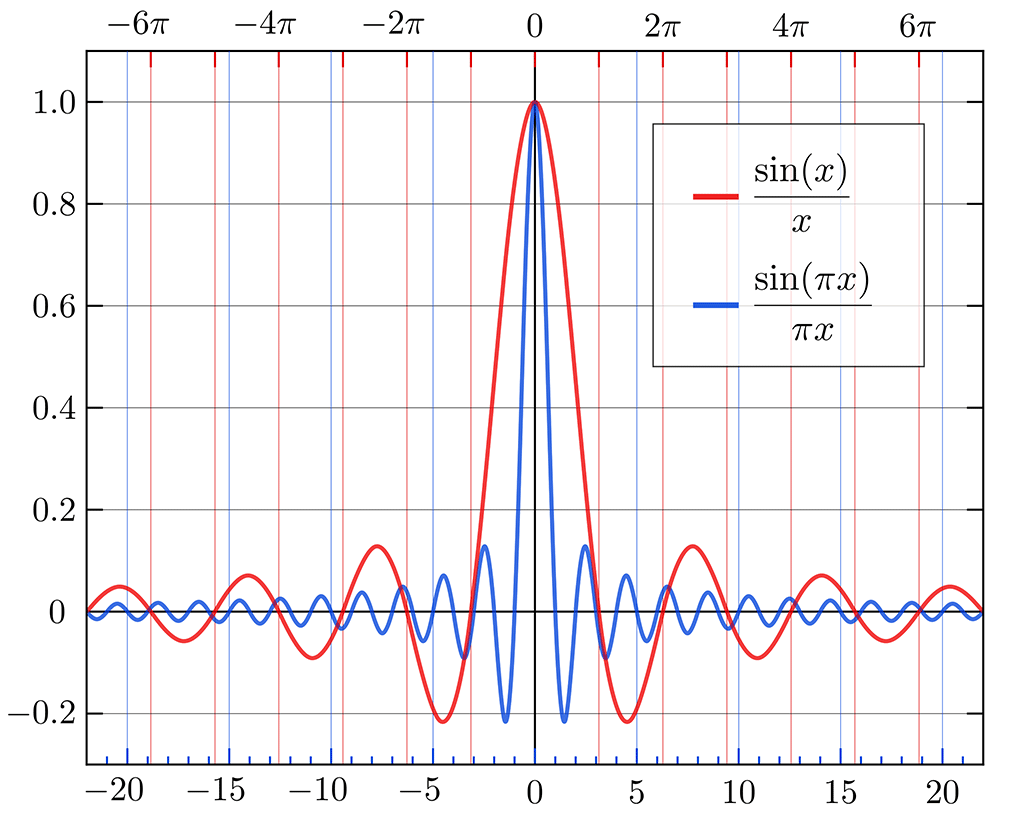
The sinc function can be expressed in unnormalized form (sin(x)/x which integral over the real line is pi) or in normalized form (sin(pi*x)/(pi*x) which integral over the real line is 1).
In both cases there is an indetermination at x=0 but you can use L’Hôpital’s rule to show that sinc(0)=1.
From Wikipedia
Fourier Transform of a rectangular shape
Since the FT is separable as mentioned above, the 2D FT of a square shape must be the 1D FT of a unit pulse in the x direction, followed by another 1D FT in the y direction.
Note that this would work for rectangles too, by using a different T value for each axis.
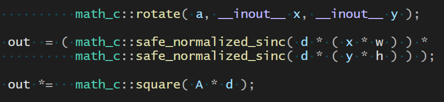
The top-right image is the actual FT of the square shape on the top-left. The bottom-right image is just the above piece of code. The bottom-left image is the profile along the x direction of the above code at y=0 which is proportional to abs(sinc).
The top-right and bottom-right images match exactly, except for:
- Some numerical drift.
- Unlike the above code, the true FT is periodic and the streaks wrap-around. But this happens to be a desirable property in my case of use.
So: success!
Can this method be generalized to n-sided polygons?
One might hope that the FT of n-sided polygons, or even inf-sided polygons (circles) could be conscructed similarly by composing rotating FTs of square functions somehow. But the truth is that things get a little bit more complicated than that.
In particular, the other case of interest for me in my application besides squares is circles. We’ll get into those in a future post.
The double-slit experiment
In the basic version of the double-slit experiment, a laser beam illuminates a plate pierced by two parallel slits, and the light passing through the slits is observed on a screen behind the plate. The wave nature of light causes the light waves passing through the two slits to interfere, producing bright and dark bands on the screen.
The pattern formed on the screen is the (constructive/destructive) sum of two rectangular interference patterns; one per slit. The profile of each pattern happens to be a sinc function.
In this image below, I have dimmed the slits vertically using a gaussian in order to generate an image that more closely resembles classic pictures of the experiment.